NSE - Native Storage extension - warm data

Data tiering has become increasingly important in the operation of SAP HANA databases in recent years. Why? Since then, more and more systems have required HANA as a prerequisite. Furthermore, data inflow has also increased significantly. There are more and more connected systems feeding data into the database. The result is unplanned growth, leading to increased resource consumption, resizing, and consequently, significantly higher operating costs.

This leads to some questions for every SAP customer running HANA systems:

1.    Do you know your operating costs per GB of RAM?

2.    Do you know your inflow and outflow of data per year?

3.    How long will your sizes continue to meet the requirements?

4.    Are you fully utilizing your data tiering capabilities?

These questions ultimately lead to an important question due to the recent changes in legislation: Do you know the CO2 emissions per system and is your measurement suitable for an audit under the CSRD (Sustainable Corporate Reporting Directive)?

But first things first: What exactly is meant by data tiering in the SAP universe? Looking at the SAP documentation (*1, *2, *3) quickly leads to the topic of multi-temperature storage strategy.

SAP defines this as:

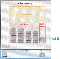
1.    Hot Data: Column Store (HANA in-memory)

2.    Warm Data: NSE (Native Storage Extension) or Extension Nodes (BW scale-out)

3.    Cold Data: Data Tiering with external storage such as NLS (Near-Line Storage)

At XLC, we take data tiering a step further, focusing on the optimal utilization of available resources. Ultimately, this allows us to optimize current sizing without the need to purchase expensive new hardware.

What approaches or features do we use for this, in addition to the well-known NSE and NLS?

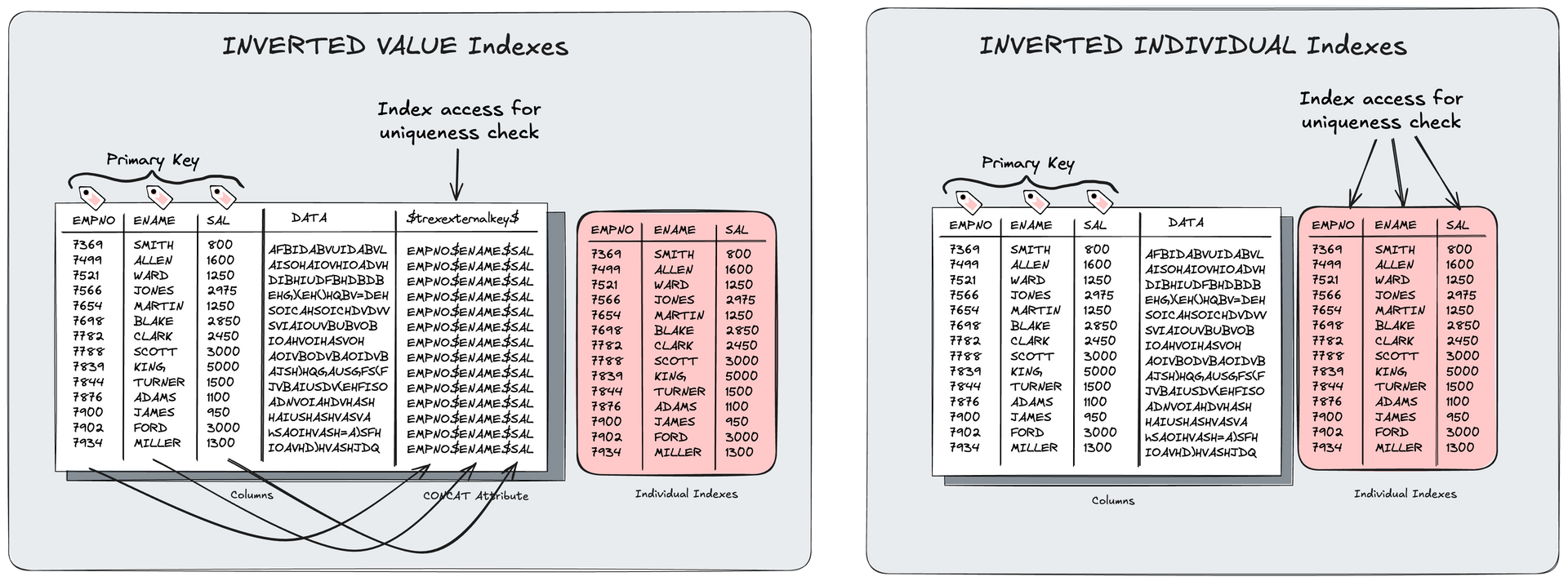
• Use of Inverted Individual Indexes (optimized indexes without significant persistence overhead)
• Use of Workload Management (restricting resources on unimportant processes and prioritizing important/critical processes), including HANA parameterization
• Optimization of partitioning (avoiding suboptimal dictionaries through multi-column designs)
• BW: Optimization of key fields and concat attributes
• Deletion of unnecessary indexes from anyDB time
• Correct sizing without peak sizing (=SAP sizing report)
• VARBINARY to LOB conversion
• and many more

We are dividing our data tiering projects into 2-3 phases:

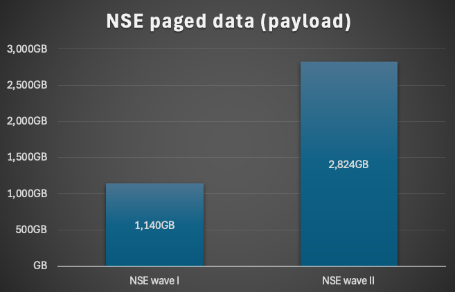
• NSE wave I: technical tables (discovery phase with health checks and implementation of uncritical tables)
• NSE wave II: business tables (conservative variant)
• review / change design (aggressive variant)

In one of our projects last year, we could achieve impressive savings on multiple systems. The following case study summary provides an overview of the challenge the client faced, how we achieved the savings, and the ultimate impact of all measures on costs.

Customer case

Environment:

• 5x SAP production systems (~15TB)
• 10x HSR (secondary and tertiary of production systems) (~30TB)
• 10x SAP non-production systems (~20TB)
• Platform: AS Azure (Europe: Amsterdam)

Challenge:

• rising costs
• high data inflow rates
• no data tiering strategy

Goals:

• optimizing instance costs
• create proper sizing forecast
• no performance impact for business-critical workload
• legal retention obligations
• proper scaling of systems
• Low-effort operating concept

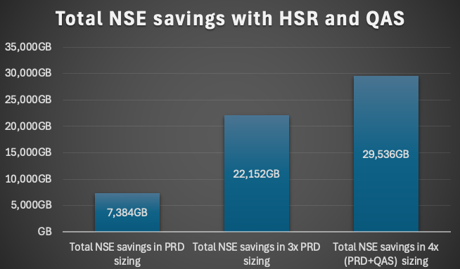
This means a reduction of the sizing results in a factor x4 for this environment. 3x PRD (primary, secondary and tertiary) + 1 QAS

Phase 1

In the first phase we created a system health check, analysed the workload and created a sizing. As part of this phase the technical tables (=NSE wave I) which normally are not part of critical workload are activated for NSE. The workload will be divided into business-critical and uncritical. Peaks will be analysed and mapped to workload classes if needed or optimized. This data will be used for phase 2 and the business-critical workload. A mapping together with the customer is elementary to prioritize and question the workload in detail.

Duration until implementation in production for technical tables (=NSE wave I): 4 weeks

Phase 2

The SQLs of each object business-critical will be analysed with a heatmap. A design with different variants will be created based on the details like SQL where clauses, CPU / memory resources, usage of indexes, materialization of columns, read and write rates. Mostly a moderate design with low risk will be used as design in this phase.

Duration until implementation in production (=NSE wave II): 6 weeks

Phase 3

After implementing the designs, the review of the performance, calculate the sizing and a forecast are part of it. If a design has a massive negative impact to the performance, a fallback to the old design hast to be done. Over time the design can also be adapted from conservative, moderate to aggressive.

NSE wording definitions

To interpret all figures correct you have to differ some of them and define the meaning and how they are calculated.

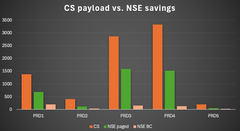
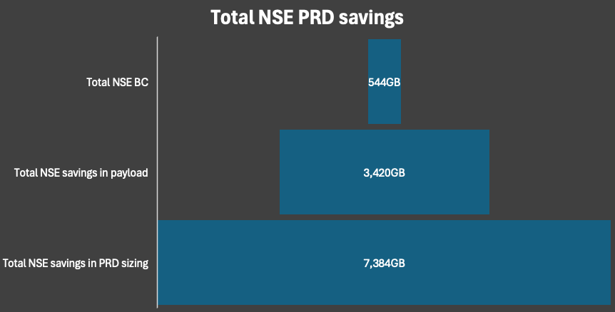
CS payload = all CS data in the system

NSE BC = NSE buffer cache

Paged data = CS data (payload) paged out as NSE data

NSE payload savings = paged data – NSE BC

NSE savings in sizing = paged data * 2 – NSE BC

Results and savings

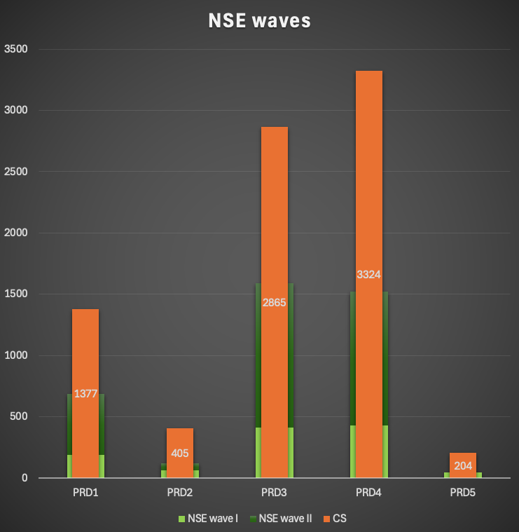
In average the CS payload could be reduced by 41%. For one system we could reduce the payload by 56%! This is called the amount of paged data, but in the end not the savings:

• PRD1: 50%
• PRD2: 30%
• PRD3: 56%
• PRD4: 46%
• PRD5: 23%
• 
  

Only considering the reduction in the productive systems we could achieve a total NSE paged data of about 4TB. Since all systems were replicated twice the savings could be tripled.

The NSE paged data of the payload represents not the saving within the sizing. Due to the fact that for the SAP sizing the CS payload will be doubled it would nearly double the savings. Why only nearly? You need a certain amount of NSE buffer cache which reduces the savings.

A total NSE saving of more than 7TB for the 5 productive systems could be achieved. This is a moving target because this was the snapshot at the time of measurement. Due to the inflow of data we already reached 8TB of savings after 6 months. This means it is not an one time saving. It will help you over time to reduce the HANA sizing as well.

In the end the NSE savings reached nearly 30TB considering the fact of HSR and QAS systems.

Summary

With NSE you can achieve between 30-60% of reduction of the payload. It is a quite easy method to save some memory if it is done in a structured way. There is risk to impact the performance which should always avoided – especially for the business-critical workload. In our cases the impact varied from 2 – 8%. You can also try the NSE advisor, which is free of charge, but it won’t rate your SQL workload and give you partition instructions.

Also, this means not that you can reduce the sizing by these values. This means also that you cannot easy change the instance size. You have to consider also other facts like LOB, SQL workload, inflow and outflow (archiving). If you are not considering this it will not lead to a successful project.

During our NSE phase one we are also creating a health check report for each system. In this phase we identified some SQL workload issues and some more potentials for inverted individual indexes.

The next part of the blog series will cover inverted individual indexes, HANA sizing and CO2 emission + cost calculation. Not every saving always results in an instance resizing. You have to consider the CPU load and the future growth of the system. Our sizing calculation will be covered by Arwel Owen.